2018-07-07

机器学习(Coursera - Andrew NG)个人笔记

一直觉得Coursera是个很好的学习平台, 因为课程中都会穿插着丰富的课后作业和大作业(真正掌握知识还是需要主动思考🤔和实践). 而且很巧, 四年多前刚开始写博客时, 记录的是学习《An Introduction to Interactive Programming in Python》的过程. 当时每个人的大作业都是随机五个同学批改的, 这篇博客记录了来自世界各地的人对我作业的评论😄).
四年后重新出发, 学习Andrew Ng的《Machine Learning》), 分享一下自己的笔记和小小感悟.

第一周

机器学习定义:

Well-posed Learning Problem: A computer program is said to learnfrom experience E with respect to some task T and some performance measure P, if its performance on T, as measured by P, improves with experience E.
T: Classifying emails as spam or not spam.
E: Watching u label emails as spam or not spam.
P: The number of emails correctly classified as spam.

机器学习算法分类:

Supervised Learning

• regression: 在连续的数据中预测
  
• classification: 最大的区别在于预测的结果, 肯定为yes or no, 或者一个集合内, e.g. 红, 黄, 蓝, 绿
  

Unsupervised learning

给定数据, 在不标注的情况下, automatically identify structure

• Clustering
• Non-clustering (cocktail party problem: 麦克风的分离(two audio sources))

Cost Function

linear regression:

• m = number of training examples
• (x_i, y_i) → single training example, i: index

cost function(squared error function) → measure the accuracy
a fancier version of an average: 个人理解用平方将个别差异放大.
(为什么要除以2m而不是m)??(哇, 下一节的笔记就有解释): The mean is halved(1/2) as a convenience for the computation of the gradient descent.
(没看懂, 希望之后会提及) → 求导时会多出一个2, 刚好抵消了.

linear & cost function
所以目标就是找到cost function的最小值:

太帅了..

Gradient decent

gradient decent + cost function 求导(partial derivative)之后:
为什么θ_1会多出x_i?? : 求导时的参数..

原因:
chain rule:
https://zs.symbolab.com/solver/derivative-calculator/%5Cfrac%7Bd%7D%7Bdx%7D%5Cleft(%5Cleft(3x%2B1%5Cright)%5E%7B2%7D%5Cright)

convex function(bowl shape function) → 永远只有一个最低点

batch gradient descent:

Linear Algebra Review

Matrix

1. A: [1, 3] → 1 x 2 matrix
2. A: [1, 3] → A_12 = 3

Vector 定义: n x 1 matrix

% The ; denotes we are going back to a new row.
A = [1, 2, 3; 4, 5, 6; 7, 8, 9; 10, 11, 12]

% Initialize a vector 
v = [1;2;3] 

% Get the dimension of the matrix A where m = rows and n = columns
[m,n] = size(A)

% You could also store it this way
dim_A = size(A)

% Get the dimension of the vector v 
dim_v = size(v)

% Now let's index into the 2nd row 3rd column of matrix A
A_23 = A(2,3)

一个Matrix 的加减乘除:

% Initialize matrix A and B 
A = [1, 2, 4; 5, 3, 2]
B = [1, 3, 4; 1, 1, 1]

% Initialize constant s 
s = 2

% See how element-wise addition works
add_AB = A + B 

% See how element-wise subtraction works
sub_AB = A - B

% See how scalar multiplication works
mult_As = A * s

% Divide A by s
div_As = A / s

% What happens if we have a Matrix + scalar?
add_As = A + s

两个Matrix的相乘

幸好以前线性代数学的还算认真, 但下边这个相乘还是挺有意思的, 而且会让你的code变得simple and efficient:

% Initialize matrix A 
A = [1, 2, 3; 4, 5, 6;7, 8, 9] 

% Initialize vector v 
v = [1; 1; 1] 

% Multiply A * v
Av = A * v

同上:

Vectorization

Matrix Multiplication Properties

1. A x B != B x A (not commutative)
2. (AxB)xC = Ax(BxC) (associate)
3. identity matrix: AxI = IxA
   <img style=“max-height:300px” class=“lazy” data-original="\images\blog\180707_cousera_ml\DraggedImage-15.png)

Matrix inverse

如何计算的呢? 很少有人手算了, 直接pinv(A)

% Transpose A 
A_trans = A' 

Matrix Transpose

% What is A^(-1)*A? A_invA = inv(A)*A

# 第二周:
MATLAB Online: [https://matlab.mathworks.com/](https://matlab.mathworks.com/)   
太TM难用了...

## Multiple Features:
1 feature: size → price
n features: size, bedrooms, floors, .. → price
<img style="max-height:300px" class="lazy" data-original="\images\blog\180707_cousera_ml\IMG_9321.JPG">     

**Multivariate linear regression**:
<img style="max-height:300px" class="lazy" data-original="\images\blog\180707_cousera_ml\DraggedImage-19.png">     
<img style="max-height:300px" class="lazy" data-original="\images\blog\180707_cousera_ml\DraggedImage-20.png">     

## Normalization
**Feature Scaling:**
因为不同的feature范围过大, 导致gradient decent效果太差
feature 1: -1 \<-\> 3
feature 2: -1000 \<-\>  1000

**mean normalization + feature scaling**
<img style="max-height:300px" class="lazy" data-original="\images\blog\180707_cousera_ml\DraggedImage-21.png">     
<img style="max-height:300px" class="lazy" data-original="\images\blog\180707_cousera_ml\DraggedImage-22.png">     


## alpha的选择: 
不能自动选择吗?
<img style="max-height:300px" class="lazy" data-original="\images\blog\180707_cousera_ml\DraggedImage-1.tiff">     

## Features and Polynomial Regression
Polynomial: 二次, 三次, n次方程, 多项式
<img style="max-height:300px" class="lazy" data-original="\images\blog\180707_cousera_ml\UNADJUSTEDNONRAW_thumb_4ca6.jpg">     
未来会传授, 如何自动选择适合的function.

## Normal Equation
<img style="max-height:300px" class="lazy" data-original="\images\blog\180707_cousera_ml\DraggedImage-2.tiff">     
具体的证明: [https://blog.csdn.net/Artprog/article/details/51172025](https://blog.csdn.net/Artprog/article/details/51172025)


# 第三周
这一周主要就是为了解决聚类问题, 如下图:   
<img style="max-height:300px" class="lazy" data-original="\images\blog\180707_cousera_ml/classification.png">     

## Classigication的分类
1. 只聚类为1或0(binary classification problem): `{0(negative), 1(positive)}`   
2. 聚类为一个集合(multi-classification problem): `{0, 1, 2, 3}`

## Linear regression对于聚类问题的局限性
比如下图这个例子, 最右边的点就出错了:   
<img style="max-height:200px" class="lazy" data-original="\images\blog\180707_cousera_ml\limitation.png">     

## Hypothesis Representation
### Logistic Function
所以新推出了Logistic Function(sigmoid function), 目的是为了让hypothesis的值永远在0和1之间:    
<img style="max-height:300px" class="lazy" data-original="\images\blog\180707_cousera_ml/sigmoid.png">     
**具体实现:**   
```matlab
function g = sigmoid(z)
%SIGMOID Compute sigmoid function
%   g = SIGMOID(z) computes the sigmoid of z.

% You need to return the following variables correctly 
% g = zeros(size(z));

% ====================== YOUR CODE HERE ======================
% Instructions: Compute the sigmoid of each value of z (z can be a matrix,
%               vector or scalar).


g = 1 ./ (1 + exp(-z));


% =============================================================

end

Logistic Function的值其实还有另外一个含义: 代表输出结果为1的可能性:

Decision Boundary:

Training Set:

Cost function:

Simplified Cost Function & distance

将上面的两个cost function合并为一个, 和第二周的regression类似, 总的distance就等于:

distance求导(说实话没看懂, 视频中只给了结果, 可能推到比较复杂一些):

function [J, grad] = costFunction(theta, X, y)
%COSTFUNCTION Compute cost and gradient for logistic regression
%   J = COSTFUNCTION(theta, X, y) computes the cost of using theta as the
%   parameter for logistic regression and the gradient of the cost
%   w.r.t. to the parameters.

% Initialize some useful values
m = length(y); % number of training examples

% ====================== YOUR CODE HERE ======================
% Instructions: Compute the cost of a particular choice of theta.
%               You should set J to the cost.
%               Compute the partial derivatives and set grad to the partial
%               derivatives of the cost w.r.t. each parameter in theta
%
% Note: grad should have the same dimensions as theta
%

% hypothesis:
h = sigmoid(X * theta);
J = 1/m * sum(-y.*log(h) - (1-y).*log(1-h));

grad = 1/m * sum((sigmoid(X * theta) - y) .* X);

% =============================================================

end

如何处理multi-dimension classification的问题

意思就是进行多次的二次聚类: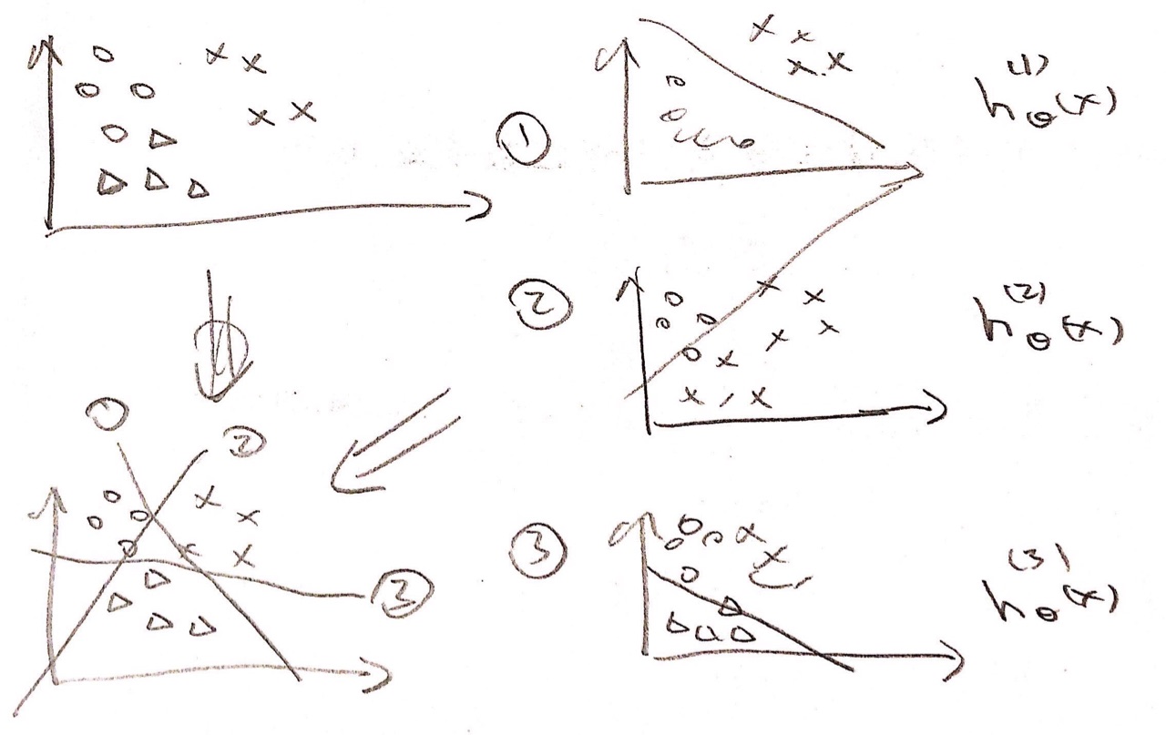

Overfitting, 意思就是说过度的拟合(没看懂, 放弃了)

很有趣的一段话:

“When I walk around Silicon Valley, I live here in Silicon Valley, there are a lot of engineers that are frankly making a ton of money for their company using machine learning algorithms. And I know we’ve only been, you know studying this stuff for a little while, But if u understand linear regression, logistic regression, the advanced optimization algorithms, and regularizaion, by now, frankly, you probably know quite a lot more machine learning than many, certainly now, but you probably know quite a lot more machine learning right now than frankly, many of the Silicon Valley engineers out there having very successful careers. You know, making tons of money for the companies. Or building products using machine learning algorithms. ”

第四周

Non-linear Hypothesis:

100 features instead of two. 50*50 pixel images → n=2500(pixels)

Quadratic features:
2500: (x_1, x_1), (x_1, x_2), (x_1, x_2), …. 2499: (x_2, x_2), (x_2, x_3), (x_2, x_3), …. … answer = 2500 + 2499 + … + 1 = 3 million

Neurons and the Brain

Neural Networks → mimic the brain 但是耗费的资源太多了, 直到最近才有比较好的计算能力去执行.

Neuron: 神经元

(brain的模拟图)

bias unit: x_0

计算第二层:
计算第三层:

乱七八糟:

编程语言: Matlab or Octave 原因:

your coding time is the most valuable resource.

matrix, vector or scalar: 矩阵, 向量, 数量

theta: θ alpha: α lambda: λ

constant e: exp(1)

slope: 斜率 converge: 收敛 derivative: 导数